Interactive Use

Basic usage

To use antelop’s interactive mode, run the command antelop-python in the terminal, either in your conda environment, or with your singularity container alias set.

This command will prompt you for your database username and password. It will then establish a connection to the database, and will open an interactive IPython shell.

There are many objects that are available to you automatically to interact with the database and your analysis functions. First of all, we have the database tables. To see what tables are available, just type:

tables

All of these tables are available for usage automatically. For example, to query the Experimenter table, just type:

Experimenter

To see a description of any table, including its attributes, and available methods, just type:

Experimenter.help()

All the analysis functions, from the standard library, your GitHub repositories and your own analysis folders are also automatically available. To see what functions are available, just type:

functions

Functions are laid out in a folder structure, with the folder names separated by dots. For example, to see all functions in the standard library, type:

stdlib

To see all functions in the script hello_world in the standard library, type:

stdlib.hello_world

Each function is accessed via its location/folder structure, separated by dots, and its name. For example, to run the function greeting() from the script hello_world in the standard library, you would type:

stdlib.hello_world.greeting()

You can additionally get information about a function including its arguments, database dependencies and description by typing:

stdlib.hello_world.greeting.help()

DataJoint Queries

You can interact with the database using DataJoint syntax. You can query the database using the following operators:

DataJoint Query Operators (source: DataJoint documentation)
operator	notation	meaning
restriction	A & cond	The subset of entities from table A that meet condition cond
restriction	A - cond	The subset of entities from table A that do not meet condition cond
join	A * B	Combines all matching information from A and B
proj	A.proj(…)	Selects and renames attributes from A or computes new attributes
aggr	A.aggr(B, …)	Same as projection but allows computations based on matching information in B
union	A + B	All unique entities from both A and B

To perform a query, you just type your query and press enter.

For example, consider the following query:

Experiment * Experimenter & 'experimenter="rbedford"'

Which gives the result:

experimenter	experiment_id	full_name	group	institution	admin	experiment_name	experiment_notes	experiment_deleted
rbedford	1	Rory Bedford	Tripodi Lab	MRC LMB	True	experiment 1	Example notes, experiment was a terrible failure.	False
rbedford	2	Rory Bedford	Tripodi Lab	MRC LMB	True	experiment 2	Experiment was a great success, I won a Nobel prize for this.	False

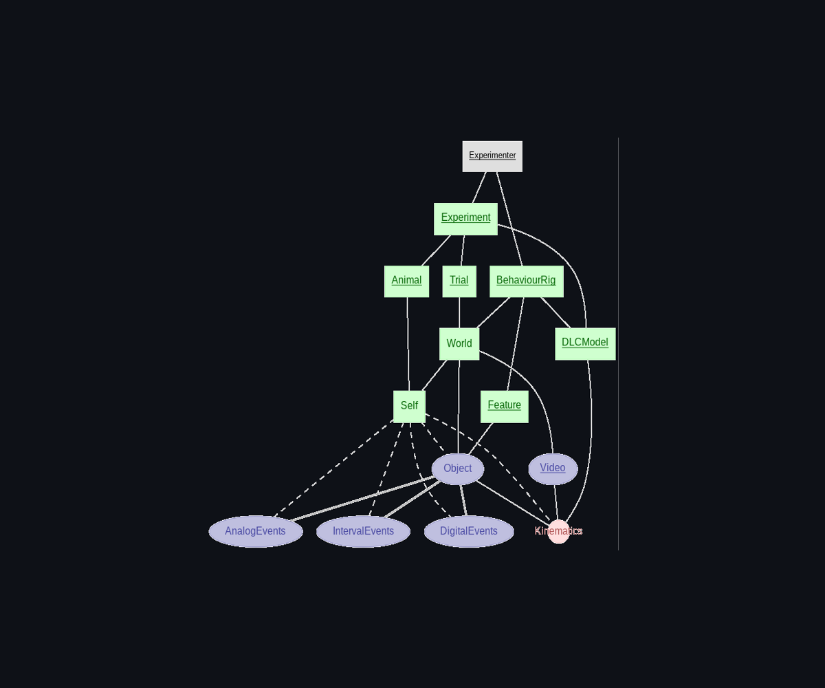
Schemas

We list show here the tables available in the database within their schema structures. To see their attributes, you can run the .help() method.

Analysis functions

Analysis functions are laid out as described in the Basic usage section. They can be run automatically on the database. For example:

stdlib.hello_world.greeting()

Will run the function greeting() from the script stdlib.hello_world, on all the data in your database. This will return a list of dictionaries, each containing the primary keys and results of the analysis function. For our lab’s database, this returns:

experimenter	greeting
arueda	Hello, Ana Gonzalez-Rueda!
dmalmazet	Hello, Daniel de Malmazet!
dwelch	Hello, Daniel Welch!
ewilliams	Hello, Elena Williams!
fmorgese	Hello, Fabio Morgese!
mtripodi	Hello, Marco Tripodi!
rbedford	Hello, Rory Bedford!
srogers	Hello, Stefan Rogers-Coltman!
yyu	Hello, Yujiao Yu!

This can be easily converted to a pandas DataFrame for further analysis as follows:

import pandas as pd
df = pd.DataFrame(stdlib.hello_world.greeting())

Analysis functions accept as their first argument a DataJoint restriction. This allows you to run the analysis on a subset of the data. They then take additional custom arguments that modify their behaviour. For example:

stdlib.hello_world.greeting({'experimenter':'rbedford'}, excited=False)

This gives:

experimenter	greeting
rbedford	Hello, Rory Bedford.

To see what keyword arguments are available, check the args attribute as follows:

stdlib.hello_world.greeting.args

To see all functions available in antelop’s standard library, see Analysis Standard Library.

Note, if you are writing analysis functions, it is useful to be able to reload them on the fly, without having to close and reopen your antelop shell. To do this, just run:

reload()

Saving function runs

Antelop provides a comprehensive framework for saving the outputs of your analysis functions in a fully reproducable manner. For details on how this works, see Reproducibility Framework. To use this framework, however, you just need to use the following function methods.

To run a function and save the output to disk, use the following method:

stdlib.hello_world.greeting.save_result(filepath='./result', format='pkl', restriction={'experimenter':'rbedford'}, excited=False)

This will save the output the output to whatever filepath you specify as a pickle file. All additional arguments and the restriction can be left blank, and the values for filepath and format we show are the defaults. A pickle file is a very fast way of saving and loading data of arbitrary types, including figures, numpy arrays, etc. To load this data at a later point, you can run:

import pandas as pd
result = pd.read_pickle('./result.pkl')

Another format you can save your data as is a csv. This is a human-readable file, so can be more useful for simple function runs. However, this method is limited by you not being able to save complex data such as figures and arrays. To save and load a csv file, you can run:

import pandas as pd
stdlib.hello_world.greeting.save_result(filepath='./result', format='csv', restriction={'experimenter':'rbedford'}, excited=False)
result = pd.read_csv('./result.csv')

All of these methods will save the output of the function, as well as a metadata file that contains all the information needed to reproduce the function run exactly. This includes the location of the function, the restriction, the arguments, and a hash of the data in the database that the function could have used. This hash is used to check that the data hasn’t changed since the function was run. For more information on how this works, see Reproducibility Framework. This metadata file is saved alongside the output file, with the same name but with the extension .json. To rerun a function from this metadata file, use:

stdlib.hello_world.greeting.reproduce(json_path='./result.json', result_path='./result.pkl')

Rerunning a function

To rerun a function from the metadata file, use the following method:

stdlib.hello_world.greeting.rerun(json_path='./result.json')

This performs all the necessary immutability checks first, and returns a warning if these fail. It then runs the function and returns the result.

Validating a function run

To manually validate the integrity of all the above factors before rerunning an analysis function, we provide the check_hash method. This takes as input just the reproducibilty json file. It checks the data_hash and code_hash against the database and function definition, and returns a message describing what’s changed, or whether you can rerun the function. For example:

hello_world.greeting.check_hash('./result.json')

Returns:

Reproducibility checks passed

Reproducing a script

A similar method to the one above reruns the analysis function and saves the results, after checking the hashes as above. This method takes in both the saved json, and an output to save results to. Execute as follows:

hello_world.greeting.reproduce('./result.json', './result.pkl')

This allows you to reproduce the results of an analysis.